Deep Dive: Analyzing Connectivity

This tutorial will guide you through the process of querying and analyzing connectivity data using the CRANTpy package. We will cover

• how to retrieve synapse data

• filter synapse data, and

• visualize the results.

Let’s get started by setting up our environment.

# Import CRANTpy and other necessary libraries
import crantpy as cp
import pandas as pd
import numpy as np
import matplotlib.pyplot as plt
import seaborn as sns
import navis 

# Set up logging to see progress
cp.set_logging_level("WARNING")
navis.set_loggers('WARNING')

print("CRANTpy loaded successfully!")
print(f"Default dataset: {cp.CRANT_DEFAULT_DATASET}")

CRANTpy loaded successfully!
Default dataset: latest

1. Authentication Setup

Before we can access the data, we need to authenticate with the CAVE service. This is typically a one-time setup.

# Generate and save authentication token (uncomment if first time)
# cp.generate_cave_token(save=True)

# Test connection
try:
    client = cp.get_cave_client()
    print(f"Successfully connected to datastack: {client.datastack_name}")
    print(f"Server: {client.server_address}")
except Exception as e:
    print(f"Connection failed: {e}")
    print("Please run: cp.generate_cave_token(save=True)")

Successfully connected to datastack: kronauer_ant
Server: https://proofreading.zetta.ai

2. Understanding Automatic ID Updates and Caching

Why ID Updates Matter

In CAVE/FlyWire, neuron segmentations are constantly being refined through proofreading. When neurons are merged or split, their root IDs change. However, the synapse tables always use the latest root IDs at the time of materialization.

This means that if you have an older root ID from a previous version, querying with it directly might:

• Return no results (if the neuron was merged into another)

• Return incomplete results (if part of it was split off)

• Give you data for the wrong neuron (if the ID now refers to something else)

Automatic ID Updates

To solve this problem, CRANTpy automatically updates all root IDs to their latest versions before querying connectivity data. This happens by default in all connectivity functions:

• get_synapses() - Updates both pre_ids and post_ids

• get_adjacency() - Updates IDs before querying synapses

• get_connectivity() - Updates neuron_ids before querying

• get_synapse_counts() - Updates neuron_ids before counting

• attach_synapses() - Updates skeleton IDs before attaching

How Caching Works

ID updates could be slow if done repeatedly, so CRANTpy uses intelligent per-ID caching:

1. Per-ID Granularity: Each individual ID’s update result is cached separately

2. Partial Reuse: If you query [ID1, ID2, ID3] and then [ID2, ID3, ID4], the cached results for ID2 and ID3 are reused

3. Automatic Expiration: Cached results expire after a configurable duration (default: 7 days)

4. Preserved Metadata: All columns (old_id, new_id, confidence, changed) are preserved in the cache

Performance Impact: For fully cached queries, you can see speedups of over 2500x! Even with partial cache hits, the overhead is minimal (1-2 seconds).

Controlling ID Updates

While automatic updates are enabled by default (update_ids=True), you can disable them if needed:

# Default behavior - IDs are automatically updated (recommended)
synapses = cp.get_synapses(pre_ids=[123, 456])

# Disable updates - only use if you're certain IDs are current
synapses = cp.get_synapses(pre_ids=[123, 456], update_ids=False)

⚠️ Warning: Only disable automatic updates if you’re absolutely certain your IDs are current. Using outdated IDs can lead to incorrect connectivity results!

# Example: See ID updates in action
import time

# Get some neuron IDs
sample_criteria = cp.NeuronCriteria(cell_class='olfactory_projection_neuron', side='right', tract='mALT')
sample_ids = sample_criteria.get_roots()[:3].astype(int).tolist()

print("First query - IDs will be updated and cached:")
start = time.time()
result1 = cp.get_synapses(pre_ids=sample_ids, threshold=5)
time1 = time.time() - start
print(f"  Query completed in {time1:.2f} seconds")
print(f"  Found {len(result1)} synapses")

print("\nSecond query - Uses cached ID updates:")
start = time.time()
result2 = cp.get_synapses(pre_ids=sample_ids, threshold=5)
time2 = time.time() - start
print(f"  Query completed in {time2:.2f} seconds")
print(f"  Found {len(result2)} synapses")

print(f"\nSpeedup from caching: {time1/time2:.1f}x faster!")
print("\nNote: The first query includes both ID update time and synapse retrieval.")
print("The second query still retrieves synapses but skips the ID update step.")

Managing Caches

If you ever need to clear the ID update cache (for example, after a new materialization), you can use:

# Clear just the ID update cache
cp.clear_global_cache('update_ids_cache')

# Clear all caches
cp.clear_all_caches()

The cache automatically expires after 7 days by default, but manual clearing can be useful if you know there have been significant proofreading changes.

3. Querying Synapses

Outputs of Olfactory Projection Neurons

Let’s start by sampling three olfactory projection neurons from the right mALT, and then use the get_synapses() function to find their postsynaptic partners.

• pre_ids=sample_ids filters for synapses downstream of our olfacotry projection neurons

• threshold=3 only preserves connections between neurons with at least 3 synapses

• materialization='latest' uses the most recent version of the synapse table

• min_size=10 thresholds on the synapse size

• return_pixels=True ensures that the coordinates in the table are in pixels, not nanometers

• update_ids=True (default) automatically updates IDs to their latest versions

# Get a sample of olfactory projection neurons
opn_criteria = cp.NeuronCriteria(cell_class='olfactory_projection_neuron', side='right', tract='mALT')
opn_ids = opn_criteria.get_roots()
print(f"Found {len(opn_ids)} olfactory projection neurons")

# Select a few for detailed analysis
sample_ids = opn_ids[:3]
print(f"\nSample neurons for detailed analysis:")
for i, neuron_id in enumerate(sample_ids, 1):
    print(f"  {i}. {neuron_id}")

# Query synapses downstream of the sample neurons
synapses = cp.get_synapses(pre_ids=sample_ids, threshold=3, materialization='latest', min_size=10, return_pixels=True).sort_values(by=['size'], ascending=False)
synapses

2025-10-09 21:21:11 - WARNING - Multiple supervoxel IDs found for 129 root IDs. Using first occurrence for each.

Found 34 olfactory projection neurons

Sample neurons for detailed analysis:
  1. 576460752773799604
  2. 576460752722298426
  3. 576460752680204173

	pre_pt_root_id	post_pt_root_id	id	created	superceded_id	valid	size	pre_pt_supervoxel_id	post_pt_supervoxel_id	pre_pt_position	post_pt_position	ctr_pt_position
2452	576460752722298426	576460752699041619	7796505	2025-03-27 13:34:35.700037+00:00	NaN	t	403	72691531949599416	72691531949596725	[11392, 11784, 3000]	[11374, 11786, 2998]	[11442, 11817, 3000]
144	576460752722298426	576460752706238547	25500275	2025-03-27 13:34:35.700037+00:00	NaN	t	375	73043375402249556	73043375402302436	[17372, 11816, 2045]	[17368, 11838, 2047]	[17374, 11836, 2052]
2604	576460752722298426	576460752765476144	20274550	2025-03-27 13:34:35.700037+00:00	NaN	t	367	72973006725106953	72973006725115267	[15480, 11684, 2279]	[15494, 11706, 2279]	[15502, 11701, 2277]
2470	576460752722298426	576460752706238547	25608007	2025-03-27 13:34:35.700037+00:00	NaN	t	329	73043375468665541	73043375468668812	[17312, 11818, 2052]	[17316, 11846, 2052]	[17332, 11844, 2055]
2569	576460752722298426	576460752756460946	45517299	2025-03-27 13:34:35.700037+00:00	NaN	t	318	73396593378155594	73396593378158596	[22152, 32672, 1431]	[22130, 32680, 1432]	[22148, 32678, 1435]
...	...	...	...	...	...	...	...	...	...	...	...	...
1062	576460752773799604	576460752690968107	75114322	2025-03-27 13:34:35.700037+00:00	NaN	t	10	74030187222317847	74030187222329021	[31622, 36238, 2531]	[31616, 36254, 2532]	[31624, 36244, 2534]
203	576460752722298426	576460752659677339	45507925	2025-03-27 13:34:35.700037+00:00	NaN	t	10	73396593378192012	73396593378194720	[22128, 32144, 1447]	[22108, 32136, 1447]	[22122, 32130, 1446]
1859	576460752773799604	576460752768105504	88939778	2025-03-27 13:34:35.700037+00:00	NaN	t	10	74450612913565186	74450612913567407	[37328, 10236, 2171]	[37310, 10212, 2173]	[37320, 10222, 2173]
1909	576460752773799604	576460752743279908	96841840	2025-03-27 13:34:35.700037+00:00	NaN	t	10	74661650627953715	74661650627966625	[40926, 8896, 2935]	[40950, 8894, 2938]	[40940, 8896, 2937]
219	576460752722298426	576460752671252568	44936261	2025-03-27 13:34:35.700037+00:00	NaN	t	10	73396524658445730	73396524658440600	[21708, 31538, 1345]	[21718, 31562, 1345]	[21724, 31550, 1345]

2998 rows × 12 columns

Let’s first count the number of synapses for each of our root IDs

synapses.groupby('pre_pt_root_id').size().reset_index(name='num_synapses')

	pre_pt_root_id	num_synapses
0	576460752680204173	801
1	576460752722298426	582
2	576460752773799604	1615

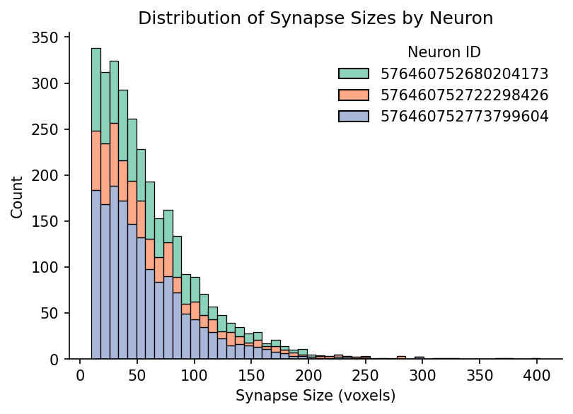
Plot distribution of synapse size

Now let’s plot the distribution of synapses sizes for each neuron

f, ax = plt.subplots(1, 1, figsize=(6, 4), dpi=150)
sns.histplot(data=synapses, x='size', hue='pre_pt_root_id', multiple='stack', bins=50, ax=ax, stat='count', legend=True, palette='Set2')
ax.set_xlabel('Synapse Size (voxels)')
ax.set_ylabel('Count')
ax.set_title('Distribution of Synapse Sizes by Neuron')
ax.spines['top'].set_visible(False)
ax.spines['right'].set_visible(False)

# Customize legend
legend = ax.get_legend()
legend.set_title('Neuron ID')  # Change legend title
legend.set_frame_on(False)     # Turn off legend frame

plt.show()

Inspect synapses in the EM data

Now let’s plot the raw EM data centered at the three largest synapses and inspect whether we see synaptic vesicles.

# Plot EM image around the detected synapses
image_size = 500
top_synapse_coords = synapses[['ctr_pt_position']].head(3).values.tolist()
fig, axes = plt.subplots(1, 3, figsize=(15, 5))
for ax, coords in zip(axes, top_synapse_coords):
    x_center, y_center, z_center = coords[0]
    img = cp.plot_em_image(x_center, y_center, z_center, size=image_size)
    ax.scatter(image_size//2, image_size//2, marker='x', color='red', s=100)
    ax.imshow(img, cmap='gray')
    ax.set_title(f"Synapse at ({x_center}, {y_center}, {z_center})")
    ax.axis('off')
plt.tight_layout()
plt.show()

Downloading Bundles: 100%|██████████| 5/5 [00:00<00:00,  5.85it/s]
Decompressing: 100%|██████████| 9/9 [00:00<00:00, 1222.67it/s]
Downloading Bundles: 100%|██████████| 5/5 [00:01<00:00,  3.29it/s]
Decompressing: 100%|██████████| 9/9 [00:00<00:00, 101.64it/s]
Downloading Bundles: 100%|██████████| 5/5 [00:03<00:00,  1.29it/s]
Decompressing: 100%|██████████| 9/9 [00:00<00:00, 45.13it/s]

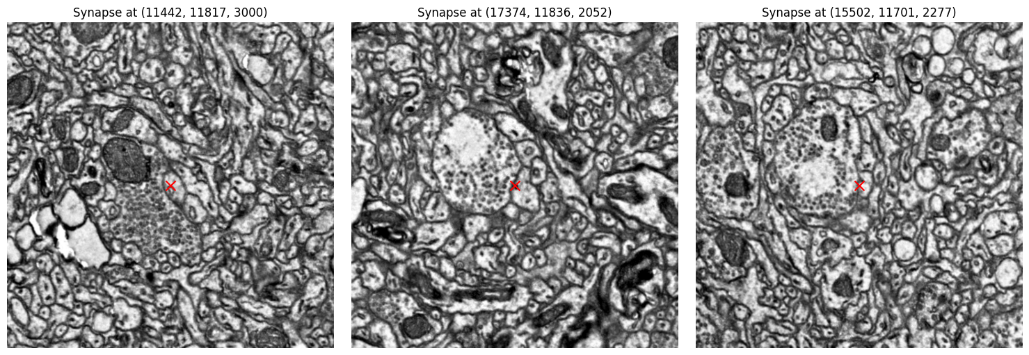
The presynaptic neurons clearly have lots of vesicles!

4. Querying Adjacency

Inputs to Olfactory Projection Neurons

Instead of getting the full synapse table, we can get an adjacency matrix of synaptic connections between neurons using the get_adjacency function:

• post_ids=sample_ids exclusively looks for inputs to the neurons

• symmetric=False ensures that rows represent pre-synaptic neurons and columns post-synaptic neurons.

• IDs are automatically updated before querying (can be disabled with update_ids=False)

# Get a sample of olfactory projection neurons
opn_criteria = cp.NeuronCriteria(cell_class='olfactory_projection_neuron', side='right', tract='mALT')
opn_ids = opn_criteria.get_roots()
sample_ids = opn_ids[:5]

# Get adjacency matrix for the sample neurons
adjacency = cp.get_adjacency(post_ids=sample_ids, threshold=3, symmetric=False)
print(f"Adjacency matrix shape: {adjacency.shape}")
print(f"Identified {adjacency.shape[0]} input neurons connected to our {adjacency.shape[1]} sample PNs.")

2025-10-09 21:21:47 - WARNING - Multiple supervoxel IDs found for 129 root IDs. Using first occurrence for each.

Adjacency matrix shape: (124, 5)
Identified 124 input neurons connected to our 5 sample PNs.

Let’s sort the rows and columns and plot a heatmap to visualize our adjacency matrix.

# Sort columns by the maximum connections
col_sums = adjacency.sum(axis=0)
sorted_indices = col_sums.sort_values(ascending=False).index
adjacency = adjacency[sorted_indices]

# sort rows by the location of their maximum connection
row_max_locs = adjacency.values.argmax(axis=1)
sorted_row_indices = np.argsort(row_max_locs)
adjacency = adjacency.iloc[sorted_row_indices]

# Plot heatmap of connections 
plt.figure(figsize=(6, 10), dpi=150)
plt.imshow(adjacency.values, aspect='auto', cmap='viridis')
plt.colorbar(label='Number of Synapses')
plt.xlabel('PNs')
plt.ylabel('Inputs')
plt.xticks(ticks=np.arange(len(adjacency.columns)), labels=adjacency.columns, rotation=0, fontsize=3)
plt.yticks(ticks=np.arange(len(adjacency.index)), labels=adjacency.index, fontsize=3)
plt.show()

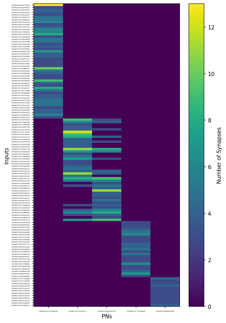
By eye, it looks like two of these PNs share the same glomerulus!

Querying Adjacency within the Central Complex

Now let’s query connectivity in the central complex.
First we will collect determine our neurons of interest using NeuronCriteria:

# Get neurons belonging to the central complex 
cx_neurons = cp.NeuronCriteria(cell_class=['EBc', 'ER', 'FBt', 'PBt'], region='CX')
print(f"Filtered to {len(cx_neurons.get_roots())} neurons in selected classes.")
cx_annotations = cp.get_annotations(cx_neurons)
cx_annotations['cell_class'].value_counts().reset_index()

Filtered to 333 neurons in selected classes.

	cell_class	count
0	ER	137
1	FBt	91
2	PBt	64
3	EBc	47

Now when we use get_adjacency we restrict both pre_ids and post_ids to our predefined NeuronCriteria to only query connections betweeen our neurons of interest.

adjacency = cp.get_adjacency(pre_ids=cx_neurons, post_ids=cx_neurons, threshold=3, symmetric=True)

2025-10-09 21:22:30 - WARNING - Multiple supervoxel IDs found for 129 root IDs. Using first occurrence for each.

And now we plot a heatmap grouped by cell class:

# Create neuron to class mapping using the existing cx_annotations
# Convert root_id to int to match adjacency matrix data type
cx_annotations_int = cx_annotations.copy()
cx_annotations_int['root_id'] = cx_annotations_int['root_id'].astype(int)
neuron_to_class = cx_annotations_int.set_index('root_id')['cell_class'].to_dict()

# Create sorted lists of neuron IDs grouped by class
class_groups = {}
for neuron_id in adjacency.index:
    cell_class = neuron_to_class.get(neuron_id, 'Unknown')
    if cell_class not in class_groups:
        class_groups[cell_class] = []
    class_groups[cell_class].append(neuron_id)

# Sort classes by number of neurons (largest first)
sorted_classes = sorted(class_groups.keys(), key=lambda x: len(class_groups[x]), reverse=True)
sorted_neuron_ids = []
for cls in sorted_classes:
    sorted_neuron_ids.extend(sorted(class_groups[cls]))

# Reorder the adjacency matrix
adjacency_sorted = adjacency.loc[sorted_neuron_ids, sorted_neuron_ids]

# Create the heatmap using seaborn
plt.figure(figsize=(8, 6), dpi=200)
ax = sns.heatmap(adjacency_sorted.values, 
                 cmap='coolwarm', 
                 cbar_kws={'label': 'Number of Synapses'},
                 square=True)

# Add class boundaries
class_boundaries = []
current_pos = 0
for cls in sorted_classes:
    current_pos += len(class_groups[cls])
    class_boundaries.append(current_pos)

# Draw lines to separate classes
for boundary in class_boundaries[:-1]:  # Don't draw the last boundary
    ax.axhline(boundary, color='white', linewidth=2, alpha=0.8)
    ax.axvline(boundary, color='white', linewidth=2, alpha=0.8)

# Create class tick labels
class_positions = []
current_pos = 0
for cls in sorted_classes:
    class_size = len(class_groups[cls])
    class_positions.append(current_pos + class_size/2)
    current_pos += class_size

# Set tick labels to show classes instead of individual neuron IDs
ax.set_xticks(class_positions)
ax.set_xticklabels([f"{cls} (n={len(class_groups[cls])})" for cls in sorted_classes], 
                   rotation=45, ha='right', fontsize=10)
ax.set_yticks(class_positions)
ax.set_yticklabels([f"{cls} (n={len(class_groups[cls])})" for cls in sorted_classes], 
                   rotation=0, fontsize=10)

# Rows are pre-synaptic neurons, columns are post-synaptic neurons. Add x and y labels 
ax.set_xlabel('Post-synaptic')
ax.set_ylabel('Pre-synaptic')

plt.title('Central Complex Connectivity Matrix')
plt.tight_layout()
plt.show()

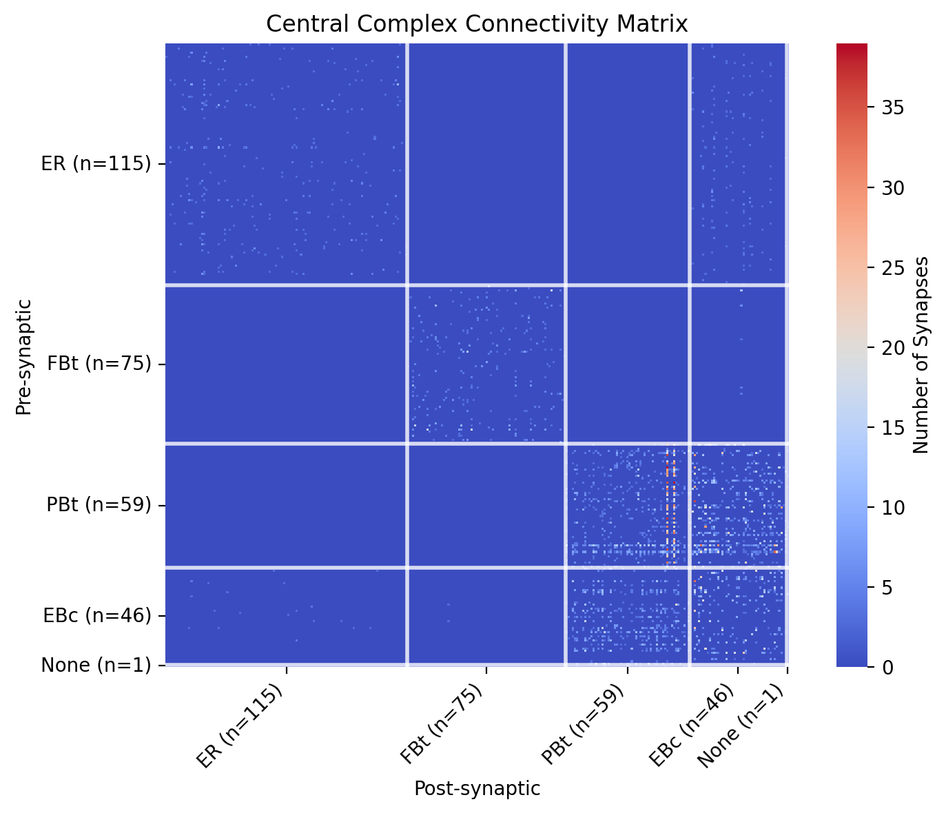
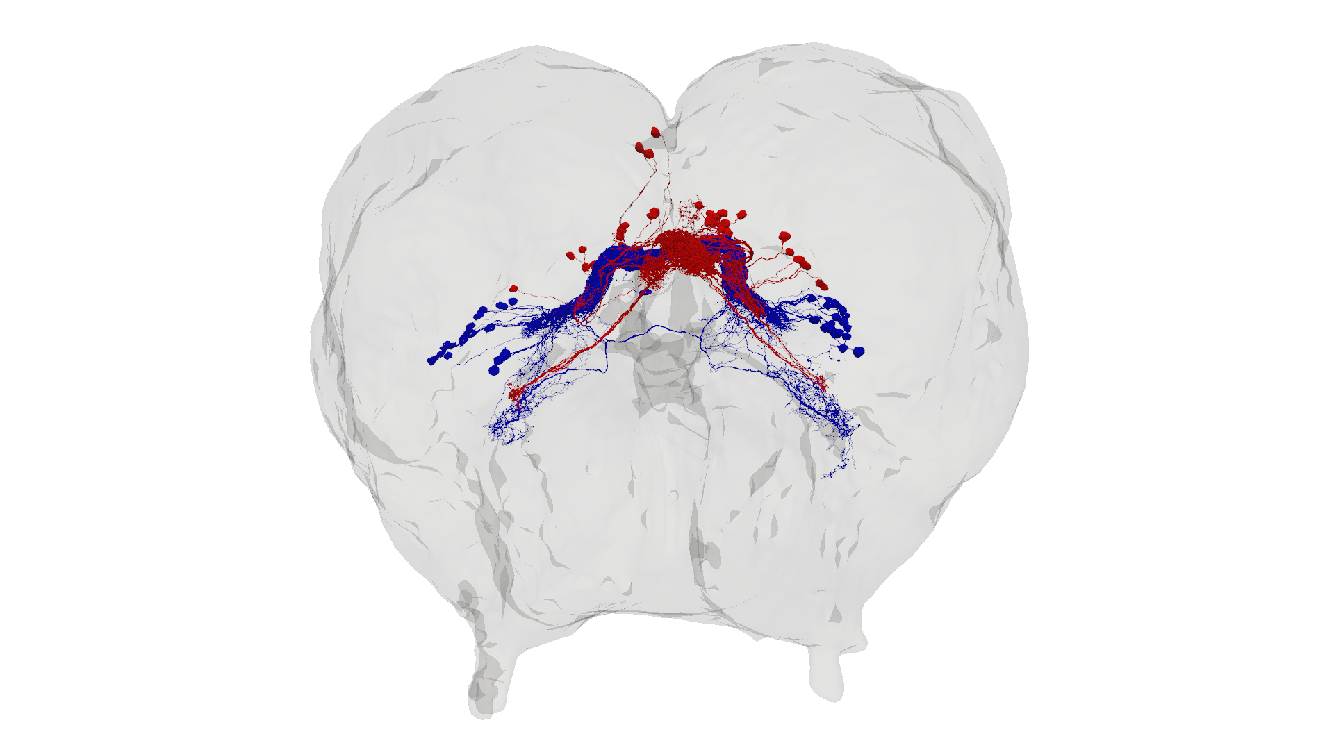
It’s clear from the heatmap that PBt and EBc populations are connected. Let’s isolate all of the EBc and PBt neurons and visualize them in the brain mesh.

# Isolate neuron subtypes 
ebc_neurons = cx_annotations[cx_annotations['cell_class'] == 'EBc']['root_id'].astype(int).tolist()
pbt_neurons = cx_annotations[cx_annotations['cell_class'] == 'PBt']['root_id'].astype(int).tolist()
print(f"Found {len(ebc_neurons)} EBc neurons and {len(pbt_neurons)} PBt neurons.")
# Combine neuron IDs
combined_ids = ebc_neurons + pbt_neurons
# Define colors 
neuron_colors = ['red' for _ in ebc_neurons] + ['blue' for _ in pbt_neurons]
# Plot the brain mesh scene
plotter = cp.get_brain_mesh_scene(combined_ids, backend='static', neuron_mesh_colors=neuron_colors) 
plotter.window_size = (1920, 1080)
plotter.zoom_camera(1.5)
plotter.show()

Found 47 EBc neurons and 64 PBt neurons.

5. Querying Connectivity

Another way of getting synapse information is using the get_connectivity function.
This function does not take a separate pre and post inputs, but you can specify whether to include upstream or downstream connections.
Here we query all of the synapses downstream and upstream of a single neuron and then plot the annotations for its connections.
Like all connectivity functions, IDs are automatically updated to their latest versions.

sample_id = 576460752732847432
print(f"Querying downstream connections for neuron ID {sample_id} of class {cp.get_annotations(sample_id)['cell_class'].values[0]}")
downstream_connections = cp.get_connectivity(neuron_ids=sample_id, upstream=False, downstream=True, threshold=5)
downstream_connections

Querying downstream connections for neuron ID 576460752732847432 of class PBt

	pre	post	weight
0	576460752732847432	576460752758099375	40
1	576460752732847432	576460752664985320	33
2	576460752732847432	576460752689030141	30
3	576460752732847432	576460752752135087	28
4	576460752732847432	576460752758006191	27
...	...	...	...
175	576460752732847432	576460752686098695	5
176	576460752732847432	576460752681077443	5
177	576460752732847432	576460752680886087	5
178	576460752732847432	576460752672839224	5
179	576460752732847432	576460752792903537	5

180 rows × 3 columns

Now we can easily add annotations, like post_cell_class, to these postsynaptic partners:

# Get annotations for postsynaptic neurons
annotations = cp.get_annotations(downstream_connections['post'].unique().tolist()).reset_index()
annotations['root_id'] = annotations['root_id'].astype(int)
# Add cell class to downstream connections, Fill in missing values with 'Unknown'
downstream_connections['post_cell_class'] = downstream_connections['post'].map(annotations.set_index('root_id')['cell_class'])
downstream_connections['post_cell_class'] = downstream_connections['post_cell_class'].fillna('Unknown')
downstream_connections

	pre	post	weight	post_cell_class
0	576460752732847432	576460752758099375	40	Unknown
1	576460752732847432	576460752664985320	33	EBc
2	576460752732847432	576460752689030141	30	EBc
3	576460752732847432	576460752752135087	28	Unknown
4	576460752732847432	576460752758006191	27	EBc
...	...	...	...	...
175	576460752732847432	576460752686098695	5	FBc
176	576460752732847432	576460752681077443	5	Unknown
177	576460752732847432	576460752680886087	5	Unknown
178	576460752732847432	576460752672839224	5	PBt
179	576460752732847432	576460752792903537	5	Unknown

180 rows × 4 columns

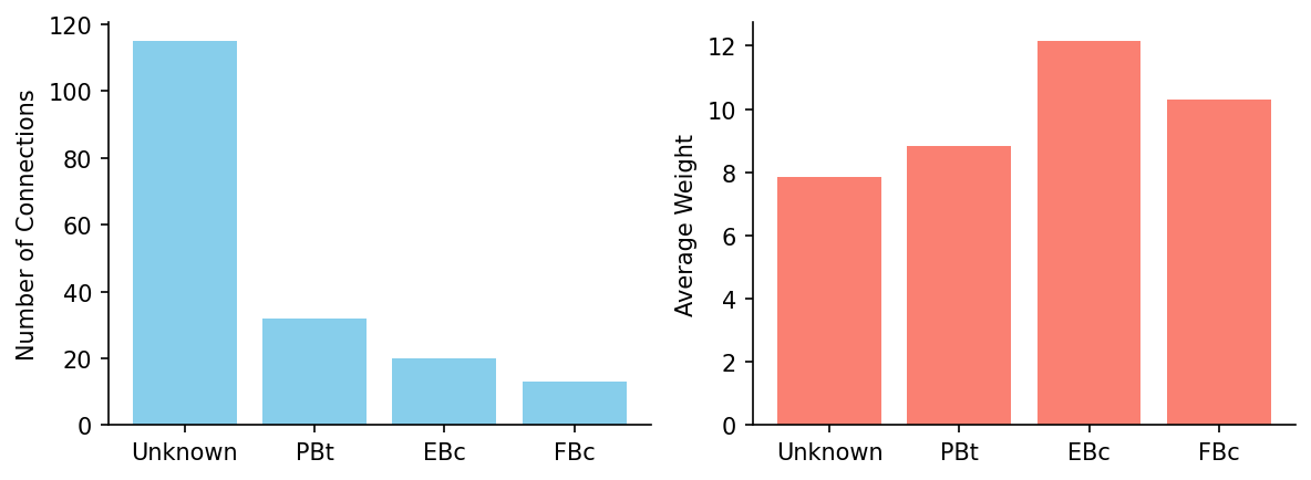
Now for each postsynaptic cell class, let’s plot the number of connections and their average weight.

# Plot number of connections and average weight by cell class
summary = downstream_connections.groupby('post_cell_class').agg(
    num_connections=('post', 'count'),
    avg_weight=('weight', 'mean')
).reset_index().sort_values(by='num_connections', ascending=False)


# Plotting 
f, ax = plt.subplots(1, 2, figsize=(8, 3), dpi=150)
ax[0].bar(summary['post_cell_class'], summary['num_connections'], color='skyblue')
ax[0].set_ylabel('Number of Connections')
ax[0].spines['top'].set_visible(False)
ax[0].spines['right'].set_visible(False)

ax[1].bar(summary['post_cell_class'], summary['avg_weight'], color='salmon')
ax[1].set_ylabel('Average Weight')
ax[1].spines['top'].set_visible(False)
ax[1].spines['right'].set_visible(False)
plt.tight_layout()
plt.show()

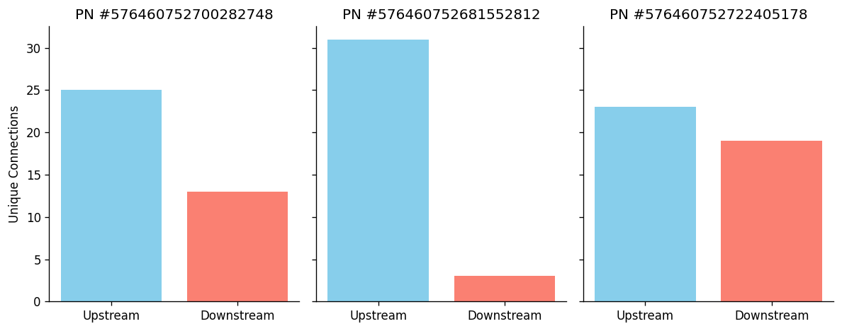
6. Synapse Counts

If we don’t care about the identity of the synaptic partners and just the number of connections, we can use the function get_synapse_counts.
Here we sample 5 olfactory projection neurons from the left mALT tract, retrieve the synapse counts and plot the number of upstream and downstream connections.
All neuron IDs are automatically updated before counting synapses.

# Get a sample of olfactory projection neurons
opn_criteria = cp.NeuronCriteria(cell_class='olfactory_projection_neuron', side='left', tract='mALT')
opn_ids = opn_criteria.get_roots()

# Select a few for synapse count analysis
sample_ids = opn_ids[:3].astype(int).tolist()
synapse_counts = cp.get_synapse_counts(neuron_ids=sample_ids, threshold=5)
synapse_counts

2025-10-09 21:26:16 - WARNING - Multiple supervoxel IDs found for 129 root IDs. Using first occurrence for each.

	pre	post
neuron_id
576460752700282748	25	13
576460752681552812	31	3
576460752722405178	23	19

fig, axes = plt.subplots(1, 3, figsize=(10, 4), sharey=True, dpi=120)
for ax, row in zip(axes, synapse_counts.iterrows()):
    upstream_count = row[1]['pre']
    downstream_count = row[1]['post']
    ax.bar(['Upstream', 'Downstream'], [upstream_count, downstream_count], color=['skyblue', 'salmon'])
    ax.set_title(f"PN #{row[0]}")
    ax.spines['top'].set_visible(False)
    ax.spines['right'].set_visible(False)
axes[0].set_ylabel('Unique Connections')
plt.tight_layout()
plt.show()