Deep Dive: Plotting Neurons

This tutorial will guide you through the process of plotting neurons using the CRANTpy library. We will cover the basics of loading neuron data, visualizing it in 2D and 3D, and customizing the plots to enhance their appearance. We introduce how to plot single neurons and multiple neurons, and how to visualize them in the context of the whole brain mesh.

# Import CRANTpy and other necessary libraries
import crantpy as cp
import pandas as pd
import numpy as np
import matplotlib.pyplot as plt
import seaborn as sns
import navis
import cloudvolume as cv
import pyvista as pv

# Set up logging to see progress
cp.set_logging_level("WARNING")
navis.set_loggers('WARNING')

print("CRANTpy loaded successfully!")
print(f"Default dataset: {cp.CRANT_DEFAULT_DATASET}")

CRANTpy loaded successfully!
Default dataset: latest

1. Authentication Setup

First, ensure you are authenticated with the CAVE service.

# Generate and save authentication token (uncomment if first time)
# cp.generate_cave_token(save=True)

# Test connection
try:
    client = cp.get_cave_client()
    print(f"Successfully connected to datastack: {client.datastack_name}")
    print(f"Server: {client.server_address}")
except Exception as e:
    print(f"Connection failed: {e}")
    print("Please run: cp.generate_cave_token(save=True)")

Successfully connected to datastack: kronauer_ant
Server: https://proofreading.zetta.ai

2. Skeletons

You can generate skeletons for neurons using the L2 chunks and CloudVolume.
The full suite of Navis visualizations and analysis functions are available once you retrieve these data types.

• The function get_l2_skeleton returns a navis.TreeNeuron or navis.NeuronList.

Generate L2 skeleton for a single neuron

Let’s start by retrieving the L2 skeleton for a single neuron.

neuron_id = 576460752664524086
skeleton = cp.get_l2_skeleton(neuron_id)
print(f"Loaded skeleton with {skeleton.n_nodes} nodes and a cable length of {skeleton.cable_length/1e6:.2f} mm.")

Loaded skeleton with 388 nodes and a cable length of 1.69 mm.

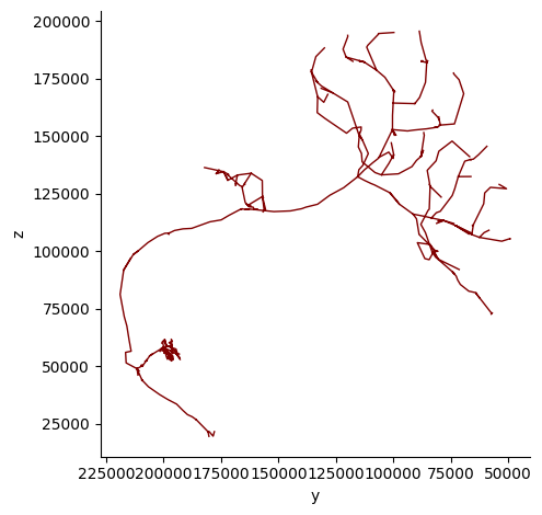
Now we can plot using plot2d and plot3d from Navis. We can specify the neuron’s color and the axes the perspective of the camera.

fig, ax = navis.plot2d(skeleton, view=("-y", "z"), color='maroon')
plt.grid(False)
ax.spines['top'].set_visible(False)
ax.spines['right'].set_visible(False)
plt.tight_layout()
plt.show()

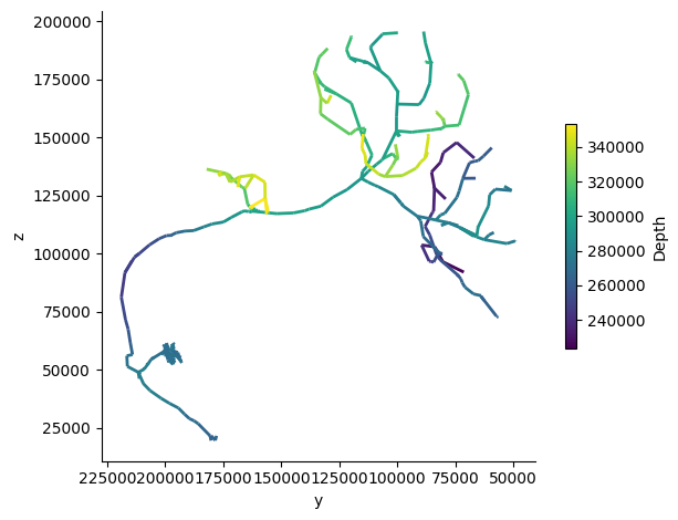
Alternatively, we can color the neuron by it’s depth (distance to camera) and increase the thickness of the skeleton line:

fig, ax = navis.plot2d(skeleton, view=("-y", "z"), depth_coloring=True, palette='viridis', linewidth=2)
plt.grid(False)
ax.spines['top'].set_visible(False)
ax.spines['right'].set_visible(False)
plt.tight_layout()
plt.show()

Generate L2 skeleton for multiple neuron

Now let’s retrieve the L2 skeleton for multiple neuron root IDs and plot them in 3D.

neuron_ids = [576460752641833774, 576460752664524086, 576460752662516321]
skeletons = cp.get_l2_skeleton(neuron_ids)

fig = skeletons.plot3d(backend='plotly', inline=False, palette='Set1')
fig.write_html('../_static/multiple_neurons_skeletons.html', include_plotlyjs="inline", full_html=True)

3. Meshes

You can also generate meshes for neurons using the CloudVolume.

• The function get_mesh_neuron returns a navis.MeshNeuron or navis.NeuronList.

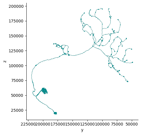
Generate mesh for a single neuron

Let’s generate a mesh for a single neuron and plot it in 2D.

neuron_id = 576460752664524086
mesh = cp.get_mesh_neuron(neuron_id)

fig, ax = navis.plot2d(mesh, view=("-y", "z"), color='darkcyan')
plt.grid(False)
ax.spines['top'].set_visible(False)
ax.spines['right'].set_visible(False)
plt.tight_layout()
plt.show()

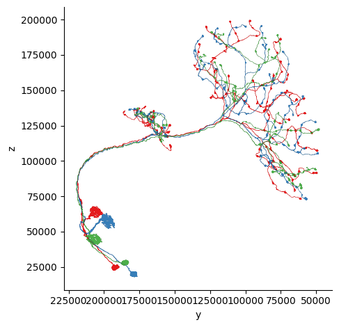
Generate mesh for multiple neuron

Now let’s retrieve the mesh for multiple neuron root IDs and plot them in 2D.

Multiple Neurons

neuron_ids = [576460752641833774, 576460752664524086, 576460752662516321]
meshes = cp.get_mesh_neuron(neuron_ids)

fig, ax = navis.plot2d(meshes, view=("-y", "z"), palette='Set1')
plt.grid(False)
ax.spines['top'].set_visible(False)
ax.spines['right'].set_visible(False)
plt.tight_layout()
plt.show()

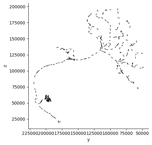
4. Dotprops

CRANTpy also allows you to use to L2 chunks to make Dotprops, point clouds with tangent vectors that are useful for NBLASTing. These can also be plotted using the same suite of functions.

• The function get_l2_dotprops returns a navis.NeuronList of navis.Dotprops.

dotprop = cp.get_l2_dotprops(neuron_id)[0]
print(f"Loaded dotprops with {dotprop.n_points} points.")

Loaded dotprops with 293 points.

fig, ax = navis.plot2d(dotprop, view=("-y", "z"), color='black')
plt.grid(False)
ax.spines['top'].set_visible(False)
ax.spines['right'].set_visible(False)
plt.tight_layout()
plt.show()

5. Combining neuron and brain mesh

Often, it is useful to visualize a neuron(s) in the context of the whole brain mesh. To do this, we have built a tool get_brain_mesh_scene that returns a pyvista Plotter object that allows for 3D rendering of neuron(s) within the whole brain mesh. It uses the get_mesh_neuron that we used above to retrieve the mesh for each neuron.

neuron_ids = [576460752641833774, 576460752664524086, 576460752662516321]
plotter = cp.get_brain_mesh_scene(neuron_ids, backend='html')
plotter.export_html("../_static/multiple_neurons_meshes_with_brain.html")