Deep Dive: Neuron Morphology Analysis

This comprehensive tutorial explores the morphological analysis capabilities of CRANTpy. We’ll cover:

1. Mesh representations - Fetching and analyzing neuron meshes

2. Skeleton representations - Multiple skeletonization methods

3. L2 graph-based skeletons - High-quality morphology from L2 chunks

4. Dotprops - Point cloud representations for fast analysis

5. Morphometric analysis - Cable length, surface area, volume, branching

6. Soma detection - Automated soma identification

7. Visualization - 2D and 3D visualization techniques

8. Population analysis - Comparing morphology across neuron groups

9. Navis integration - Leveraging navis for advanced analysis

Let’s start by setting up our environment.

# Import CRANTpy and other necessary libraries
import crantpy as cp
import pandas as pd
import numpy as np
import matplotlib.pyplot as plt
import seaborn as sns
import navis
import cloudvolume as cv
import networkx as nx

# Set up logging
cp.set_logging_level("WARNING")

print("CRANTpy loaded successfully!")
print(f"Default dataset: {cp.CRANT_DEFAULT_DATASET}")
print(f"Navis version: {navis.__version__}")

CRANTpy loaded successfully!
Default dataset: latest
Navis version: 1.10.0

1. Authentication Setup

First, ensure you are authenticated with the CAVE service.

# Generate and save authentication token (uncomment if first time)
# cp.generate_cave_token(save=True)

# Test connection
try:
    client = cp.get_cave_client()
    print(f"Successfully connected to datastack: {client.datastack_name}")
    print(f"Server: {client.server_address}")
except Exception as e:
    print(f"Connection failed: {e}")
    print("Please run: cp.generate_cave_token(save=True)")

Successfully connected to datastack: kronauer_ant
Server: https://proofreading.zetta.ai

2. Getting Sample Neurons

Let’s query some neurons for our morphology analysis.

# Get a sample of olfactory projection neurons
opn_criteria = cp.NeuronCriteria(cell_class='olfactory_projection_neuron')
opn_ids = opn_criteria.get_roots()
print(f"Found {len(opn_ids)} olfactory projection neurons")

# Select a few for detailed analysis
sample_ids = opn_ids[:3]
print(f"\nSample neurons for detailed analysis:")
for i, neuron_id in enumerate(sample_ids, 1):
    print(f"  {i}. {neuron_id}")

Found 107 olfactory projection neurons

Sample neurons for detailed analysis:
  1. 576460752700282748
  2. 576460752681552812
  3. 576460752722405178

3. Mesh Representations

Meshes provide the most detailed representation of neuron morphology, capturing the full 3D surface.

Fetching Mesh Neurons

# Fetch a single mesh neuron
single_mesh = cp.get_mesh_neuron(sample_ids[0])
print(f"Mesh neuron properties:")
print(f"  ID: {single_mesh.id}")
print(f"  Vertices: {len(single_mesh.vertices):,}")
print(f"  Faces: {len(single_mesh.faces):,}")
print(f"  Volume: {single_mesh.volume:.2f} cubic nanometers")

Mesh neuron properties:
  ID: 576460752700282748
  Vertices: 238,432
  Faces: 478,609
  Volume: 135639679325.33 cubic nanometers

# Fetch multiple mesh neurons
mesh_neurons = cp.get_mesh_neuron(sample_ids, threads=3, progress=True)
print(f"\nFetched {len(mesh_neurons)} mesh neurons")

# Summary of meshes
for n in mesh_neurons:
    print(f"  {n.id}: {len(n.vertices):,} vertices, {n.volume:.2f} μm³")

Fetched 3 mesh neurons
  576460752700282748: 238,432 vertices, 135639679325.33 μm³
  576460752681552812: 309,633 vertices, 192266769082.67 μm³
  576460752722405178: 248,290 vertices, 154247730149.33 μm³

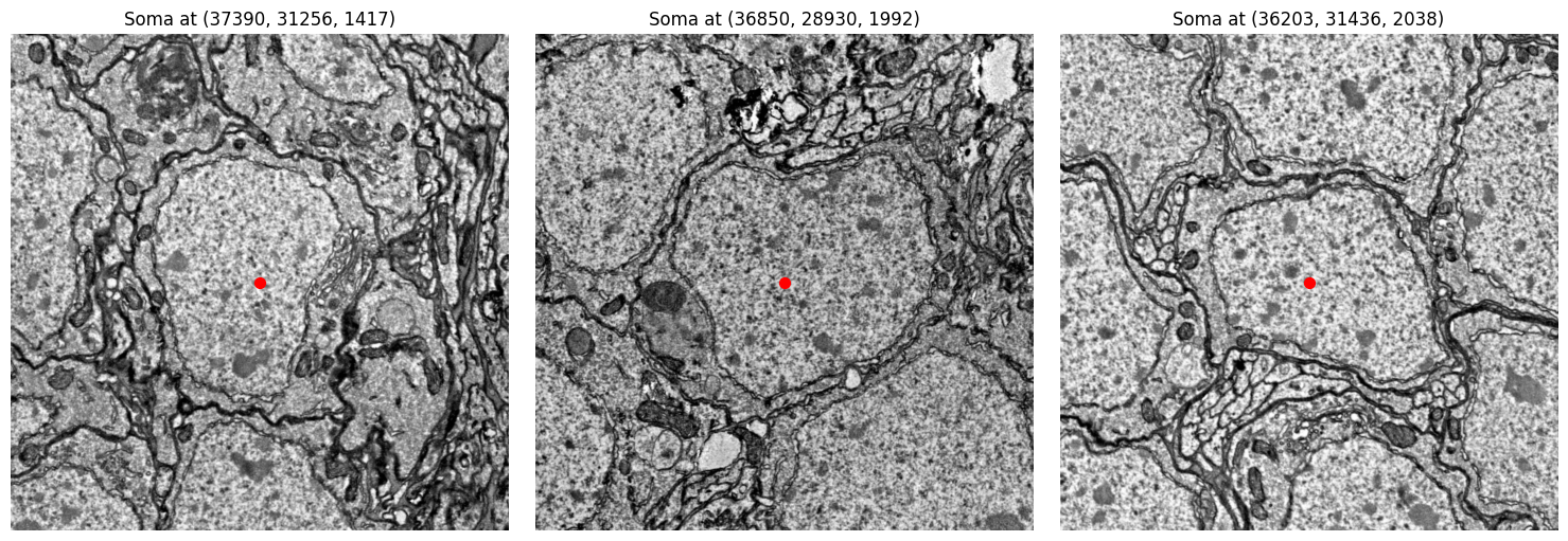
Soma Detection

We can use the function detect_soma to retrieve the estimated pixel coordinates of a neuron’s soma. We can then use a helper function to visually inspect this area in the raw EM data to verify it contains a nucleus.

# Detect soma for a single neuron
soma_coords = cp.detect_soma(sample_ids[0])
print(f"Soma detected at coordinates: {soma_coords}")

# Detect soma for multiple neurons
soma_coords_batch = cp.detect_soma(sample_ids, progress=True)
print(f"\nSoma coordinates for {len(sample_ids)} neurons:")
for neuron_id, coords in zip(sample_ids, soma_coords_batch):
    print(f"  {neuron_id}: {coords}")

Soma detected at coordinates: [37390 31256  1417]

Detecting soma:   0%|          | 0/3 [00:00<?, ?it/s]

Detecting soma:  33%|███▎      | 1/3 [00:04<00:09,  4.58s/it]

Detecting soma:  67%|██████▋   | 2/3 [00:12<00:06,  6.37s/it]

Soma coordinates for 3 neurons:
  576460752700282748: [37390 31256  1417]
  576460752681552812: [36850 28930  1992]
  576460752722405178: [36203 31436  2038]

# Plot EM image around the detected somas
fig, axes = plt.subplots(1, 3, figsize=(15, 5))
for ax, coords in zip(axes, soma_coords_batch):
    x, y, z = map(int, coords)
    img = cp.plot_em_image(x, y, z, size=1000)
    ax.scatter(500, 500, color='red', s=50)
    ax.imshow(img, cmap='gray')
    ax.set_title(f"Soma at ({x}, {y}, {z})")
    ax.axis('off')
plt.tight_layout()
plt.show()

Downloading Bundles: 100%|██████████| 11/11 [00:01<00:00, 10.24it/s]
Decompressing: 100%|██████████| 25/25 [00:00<00:00, 1361.45it/s]
Shard Indices: 100%|██████████| 4/4 [00:00<00:00, 35.14it/s]
Minishard Indices: 100%|██████████| 4/4 [00:00<00:00, 20.68it/s]
Downloading Bundles: 100%|██████████| 10/10 [00:00<00:00, 10.36it/s]
Decompressing: 100%|██████████| 20/20 [00:00<00:00, 904.64it/s]
Downloading Bundles: 100%|██████████| 11/11 [00:00<00:00, 13.35it/s]
Decompressing: 100%|██████████| 25/25 [00:00<00:00, 1505.21it/s]

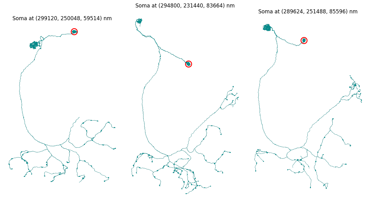
We can also plot the soma location on the mesh, but for this we need to convert from pixels coordinates to nanometers.

from crantpy.utils.config import SCALE_X, SCALE_Y, SCALE_Z
scaling_factors = np.array([SCALE_X, SCALE_Y, SCALE_Z])  # in microns

fig, ax = plt.subplots(1, 3, figsize=(12, 8))
for i in range(3):
    # scale soma coordinates to nanometers
    soma_nm = [soma_coords_batch[i][0] * SCALE_X, soma_coords_batch[i][1] * SCALE_Y, soma_coords_batch[i][2] * SCALE_Z]
    # get the mesh
    mesh = mesh_neurons[i]
    # plot the mesh with soma location
    navis.plot2d(mesh, view=("x", "y"), color='darkcyan', ax=ax[i])
    plt.grid(False)
    ax[i].set_axis_off()
    ax[i].scatter(soma_nm[0], soma_nm[1], color='red', s=200, marker='o', linewidth=2, facecolors='none')
    ax[i].set_title(f"Soma at ({int(soma_nm[0])}, {int(soma_nm[1])}, {int(soma_nm[2])}) nm", fontsize=12)
plt.tight_layout()
plt.show()

4. Skeleton Representations

Skeletons are tree-like representations that capture the branching structure of neurons while being much more computationally efficient than meshes.

Precomputed Skeletons

CRANTpy provides access to precomputed skeletons stored in the database.

# Fetch precomputed skeletons
skeletons = cp.get_skeletons(sample_ids, progress=True, omit_failures=True)
print(f"Fetched {len(skeletons)} skeletons")

# Examine first skeleton
if len(skeletons) > 0:
    skel = skeletons[0]
    print(f"\nSkeleton {skel.id} properties:")
    print(f"  Nodes: {skel.n_nodes:,}")
    print(f"  Cable length: {skel.cable_length:.2f} nm")
    print(f"  Branch points: {skel.n_branch_points}")
    print(f"  End points: {skel.n_endpoints}")

Fetched 3 skeletons

Skeleton 576460752700282748 properties:
  Nodes: 221
  Cable length: 1075895.12 nm
  Branch points: 0
  End points: None

L2 Graph-Based Skeletons

For higher quality morphology, CRANTpy can generate skeletons from L2 chunks. These are often more accurate than precomputed skeletons.

# Get L2 skeleton for a single neuron
l2_skel = cp.get_l2_skeleton(sample_ids[0], refine=True, progress=True)
print(f"L2 skeleton properties:")
print(f"  Nodes: {l2_skel.n_nodes:,}")
print(f"  Cable length: {l2_skel.cable_length:.2f} nm")
print(f"  Branch points: {l2_skel.n_branch_points}")
print(f"  End points: {l2_skel.n_endpoints}")

L2 skeleton properties:
  Nodes: 309
  Cable length: 1409182.00 nm
  Branch points: 55
  End points: None

# Get L2 skeletons for multiple neurons
l2_skels = cp.get_l2_skeleton(
    sample_ids,
    refine=True,
    progress=True,
    max_threads=3,
    omit_failures=True
)
print(f"\nFetched {len(l2_skels)} L2 skeletons")

# Compare with precomputed skeletons
if len(skeletons) > 0 and len(l2_skels) > 0:
    print(f"\nComparison (first neuron):")
    print(f"  Precomputed: {skeletons[0].cable_length:.2f} nm")
    print(f"  L2-based:    {l2_skels[0].cable_length:.2f} nm")

Fetched 3 L2 skeletons

Comparison (first neuron):
  Precomputed: 1075895.12 nm
  L2-based:    1409182.00 nm

L2 Information and Statistics

You can query L2 chunk information directly for fast morphology estimates. Note that the length_um is an underestimated sum of max diameters across L2 chunks, not a full cable length.

# Get L2 info (fast estimate of morphology)
l2_info = cp.get_l2_info(sample_ids[:5], progress=True)
print("L2 chunk information:")
display(l2_info[['root_id', 'l2_chunks', 'length_um', 'chunks_missing']])

L2 chunk information:

	root_id	l2_chunks	length_um	chunks_missing
0	576460752722405178	377	45.559	0
1	576460752681552812	390	53.886	0
2	576460752700282748	309	39.526	0

# Get detailed L2 chunk info
l2_chunk_info = cp.get_l2_chunk_info(sample_ids[0], progress=True)
print(f"\nDetailed L2 chunk info for neuron {sample_ids[0]}:")
print(f"  Total chunks: {len(l2_chunk_info)}")
print(f"  Columns: {list(l2_chunk_info.columns)}")
display(l2_chunk_info.head())

Detailed L2 chunk info for neuron 576460752700282748:
  Total chunks: 309
  Columns: ['root_id', 'l2_id', 'x', 'y', 'z', 'vec_x', 'vec_y', 'vec_z', 'size_nm3']

	root_id	l2_id	x	y	z	vec_x	vec_y	vec_z	size_nm3
0	576460752700282748	145804519643567814	27616	9700	2815	0.404541	0.913086	0.054138	138808320
1	576460752700282748	145804519710680256	27586	9700	2816	-0.446289	0.60791	0.656738	483076608
2	576460752700282748	145804588430144816	27138	10418	3038	-0.220215	0.436035	0.872559	1065555456
3	576460752700282748	145804588497240618	27602	11262	3151	0.640625	0.618652	0.455078	568780800
4	576460752700282748	145804657216724259	27596	11264	3151	0.862305	0.304199	0.405029	333666816

Finding Anchor Locations

Find representative coordinates (in pixels) for neurons (useful for annotations or quick localization).

# Find anchor locations
anchor_locs = cp.find_anchor_loc(sample_ids, progress=True)
print("Anchor locations:")
display(anchor_locs)

Anchor locations:

	root_id	x	y	z
0	576460752700282748	37256	31210	1415
1	576460752681552812	36862	29080	1987
2	576460752722405178	36214	31498	2047

Rerooting Skeletons to the Soma

By default, skeletons may not be rooted at the soma. We can reroot them using the detected soma location.

# need to reroot the skeleton to the soma location
for i in range(3):
    skel = l2_skels[i]
    coords = soma_coords_batch[i] * scaling_factors  # scale to nm 
    node_positions = skel.nodes[['x', 'y', 'z']].values
    dists = np.linalg.norm(node_positions - coords, axis=1)
    nearest_node_idx = np.argmin(dists)
    nearest_node_id = skel.nodes.iloc[nearest_node_idx]['node_id']
    print(f"Rerooting skeleton {skel.id} at nearest node {nearest_node_id} to soma location {coords} at distance {dists[nearest_node_idx]:.2f} nm")
    skel.reroot(nearest_node_id, inplace=True)

Rerooting skeleton 576460752700282748 at nearest node 223 to soma location [299120 250048  59514] at distance 1136.51 nm
Rerooting skeleton 576460752681552812 at nearest node 276 to soma location [294800 231440  83664] at distance 346.00 nm
Rerooting skeleton 576460752722405178 at nearest node 239 to soma location [289624 251488  85596] at distance 516.06 nm

5. Dotprops - Point Cloud Representations

Dotprops are lightweight point cloud representations with tangent vectors, ideal for NBLAST comparisons.

# Generate dotprops from L2 chunks
dotprops = cp.get_l2_dotprops(
    sample_ids,
    progress=True,
    omit_failures=True
)
print(f"Generated {len(dotprops)} dotprops")

if len(dotprops) > 0:
    dp = dotprops[0]
    print(f"\nDotprop {dp.id} properties:")
    print(f"  Points: {len(dp.points)}")
    print(f"  Has vectors: {dp.vect is not None}")

Generated 3 dotprops

Dotprop 576460752700282748 properties:
  Points: 241
  Has vectors: True

6. Morphometric Analysis

Navis provides extensive morphometric analysis capabilities. Let’s explore key metrics.

Basic Morphometrics

# Use L2 skeletons for morphometric analysis
if len(l2_skels) > 0:
    morphometrics = []
    
    for skel in l2_skels:
        metrics = {
            'root_id': skel.id,
            'cable_length_nm': skel.cable_length,
            'n_nodes': skel.n_nodes,
            'n_branch_points': skel.n_branch_points,
            'n_endpoints': skel.n_endpoints,
            'n_branches': len(skel.small_segments),
        }
        morphometrics.append(metrics)
    
    morph_df = pd.DataFrame(morphometrics)
    print("Basic morphometrics:")
    display(morph_df)

Basic morphometrics:

	root_id	cable_length_nm	n_nodes	n_branch_points	n_endpoints	n_branches
0	576460752700282748	1409182.000	309	55	None	152
1	576460752681552812	1831399.000	390	68	None	183
2	576460752722405178	1539621.375	377	70	None	203

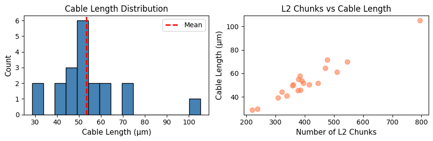
Population-Level Morphological Analysis

Let’s analyze morphology across a population of neurons.

# Get a larger sample of neurons
opn_sample = opn_ids[:20]

# Get L2 info (fast morphology estimate)
population_l2_info = cp.get_l2_info(opn_sample, progress=True)

print(f"Population morphology statistics:")
print(f"\nCable length (μm):")
print(f"  Mean: {population_l2_info['length_um'].mean():.2f}")
print(f"  Std: {population_l2_info['length_um'].std():.2f}")
print(f"  Range: {population_l2_info['length_um'].min():.2f} - {population_l2_info['length_um'].max():.2f}")

print(f"\nL2 chunks:")
print(f"  Mean: {population_l2_info['l2_chunks'].mean():.0f}")
print(f"  Range: {population_l2_info['l2_chunks'].min():.0f} - {population_l2_info['l2_chunks'].max():.0f}")

Population morphology statistics:

Cable length (μm):
  Mean: 53.39
  Std: 16.61
  Range: 28.83 - 105.19

L2 chunks:
  Mean: 406
  Range: 220 - 795

# Visualize population morphology distribution
fig, axes = plt.subplots(1, 2, figsize=(9, 3))

# Cable length distribution
axes[0].hist(population_l2_info['length_um'], bins=15, color='steelblue', edgecolor='black')
axes[0].set_xlabel('Cable Length (μm)', fontsize=11)
axes[0].set_ylabel('Count', fontsize=11)
axes[0].set_title('Cable Length Distribution', fontsize=12)
axes[0].axvline(population_l2_info['length_um'].mean(), color='red', linestyle='--', linewidth=2, label='Mean')
axes[0].legend()

# L2 chunks vs cable length
axes[1].scatter(population_l2_info['l2_chunks'], population_l2_info['length_um'], 
                color='coral', s=50, alpha=0.6)
axes[1].set_xlabel('Number of L2 Chunks', fontsize=11)
axes[1].set_ylabel('Cable Length (μm)', fontsize=11)
axes[1].set_title('L2 Chunks vs Cable Length', fontsize=12)

plt.tight_layout()
plt.show()

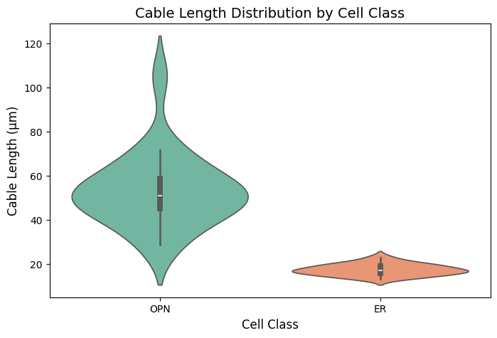
Comparing Cell Types

# Compare morphology across different cell classes
er_neurons = cp.NeuronCriteria(cell_class='ER')
er_ids = er_neurons.get_roots()[:20]

# Get L2 info for both populations
opn_morph = cp.get_l2_info(opn_sample, progress=True)
opn_morph['cell_class'] = 'OPN'

er_morph = cp.get_l2_info(er_ids, progress=True)
er_morph['cell_class'] = 'ER'

# Combine
combined_morph = pd.concat([opn_morph, er_morph], ignore_index=True)

print("Cable length statistics by cell class:")
print(combined_morph.groupby('cell_class')['length_um'].describe())

# plot the distribution of cable lengths by cell class
plt.figure(figsize=(8, 5))
sns.violinplot(x='cell_class', y='length_um', data=combined_morph, palette='Set2')
plt.title('Cable Length Distribution by Cell Class', fontsize=14)
plt.xlabel('Cell Class', fontsize=12)
plt.ylabel('Cable Length (μm)', fontsize=12)
plt.grid(False)
plt.show()

Cable length statistics by cell class:
            count     mean        std     min       25%      50%      75%  \
cell_class                                                                  
ER           20.0  17.4658   2.524752  13.349  15.96050  16.9815  19.0910   
OPN          20.0  53.3934  16.605328  28.827  45.23075  51.0715  58.7805   

                max  
cell_class           
ER           23.053  
OPN         105.185  

7. Advanced Navis Integration

CRANTpy neurons are fully compatible with navis, enabling access to its extensive analysis toolkit.

Resampling

# Resample skeleton to uniform spacing
if len(l2_skels) > 0:
    original = l2_skels[0]
    resampled = navis.resample_skeleton(original, resample_to=1000)  # 1 micron spacing
    
    print(f"Resampling:")
    print(f"  Original nodes: {original.n_nodes}")
    print(f"  Resampled nodes: {resampled.n_nodes}")
    print(f"  Original cable length: {original.cable_length:.2f} μm")
    print(f"  Resampled cable length: {resampled.cable_length:.2f} μm")

Resampling:
  Original nodes: 309
  Resampled nodes: 1317
  Original cable length: 1409182.00 μm
  Resampled cable length: 1402008.00 μm

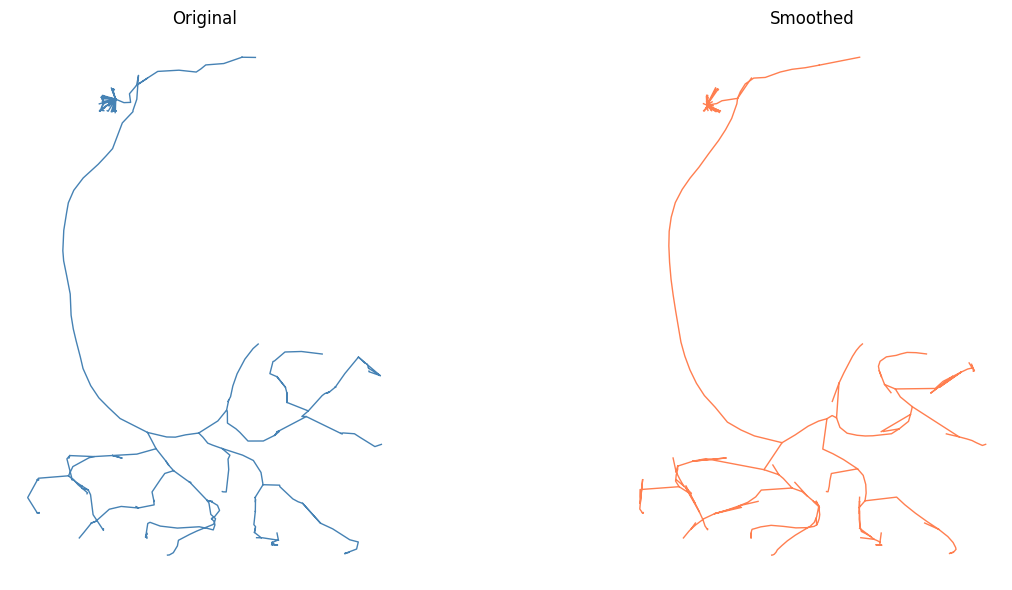
Smoothing

# Smooth skeleton
smoothed = navis.smooth_skeleton(l2_skels[0], window=5)

# Visualize original vs smoothed
fig, axes = plt.subplots(1, 2, figsize=(14, 6))

navis.plot2d(l2_skels[0], view=('x','y'), method='2d', ax=axes[0], color='steelblue')
axes[0].set_title('Original', fontsize=12)
axes[0].grid(False)
axes[0].set_axis_off()

navis.plot2d(smoothed, view=('x','y'), method='2d', ax=axes[1], color='coral')
axes[1].set_title('Smoothed', fontsize=12)
axes[1].grid(False)
axes[1].set_axis_off()

plt.tight_layout()
plt.show()

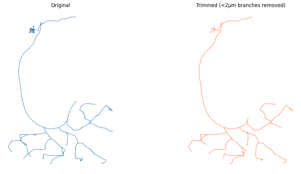
Trim branches

# trim branches shorter than a threshold
trimmed = navis.prune_twigs(l2_skels[0], size=5000*SCALE_X)
# Visualize original vs trimmed
fig, axes = plt.subplots(1, 2, figsize=(14, 6))
navis.plot2d(l2_skels[0], view=('x','y'), method='2d', ax=axes[0], color='steelblue')
axes[0].set_title('Original', fontsize=12)
axes[0].grid(False)
axes[0].set_axis_off()

navis.plot2d(trimmed, view=('x','y'), method='2d', ax=axes[1], color='coral')
axes[1].set_title('Trimmed (<2μm branches removed)', fontsize=12)
axes[1].grid(False)
axes[1].set_axis_off()
plt.tight_layout()
plt.show()

Neuron Similarity (NBLAST)

NBLAST is a powerful algorithm for quantifying morphological similarity between neurons. It operates on dotprops representations.

# get the dotprops for 30 neurons
dotprops = cp.get_l2_dotprops(
    opn_ids[:30],
    progress=True,
    omit_failures=True
)/1000 # scale to microns


# NBLAST requires dotprops
# Compute pairwise similarity
scores = navis.nblast(dotprops, dotprops).values

# Visualize similarity matrix
fig, ax = plt.subplots(figsize=(8, 7))
im = ax.imshow(scores, cmap='viridis', vmin=0, vmax=1)
ax.set_title('NBLAST Similarity Matrix', fontsize=14)
ax.set_xlabel('Neuron Index')
ax.set_ylabel('Neuron Index')
plt.colorbar(im, ax=ax, label='Normalized Score')
plt.tight_layout()
plt.show()

# Find most similar pair
np.fill_diagonal(scores, 0)  # Exclude self-comparisons
max_idx = np.unravel_index(scores.argmax(), scores.shape)
print(f"\nMost similar pair: neurons {max_idx[0]} and {max_idx[1]}")
print(f"Similarity score: {scores[max_idx]:.3f}")

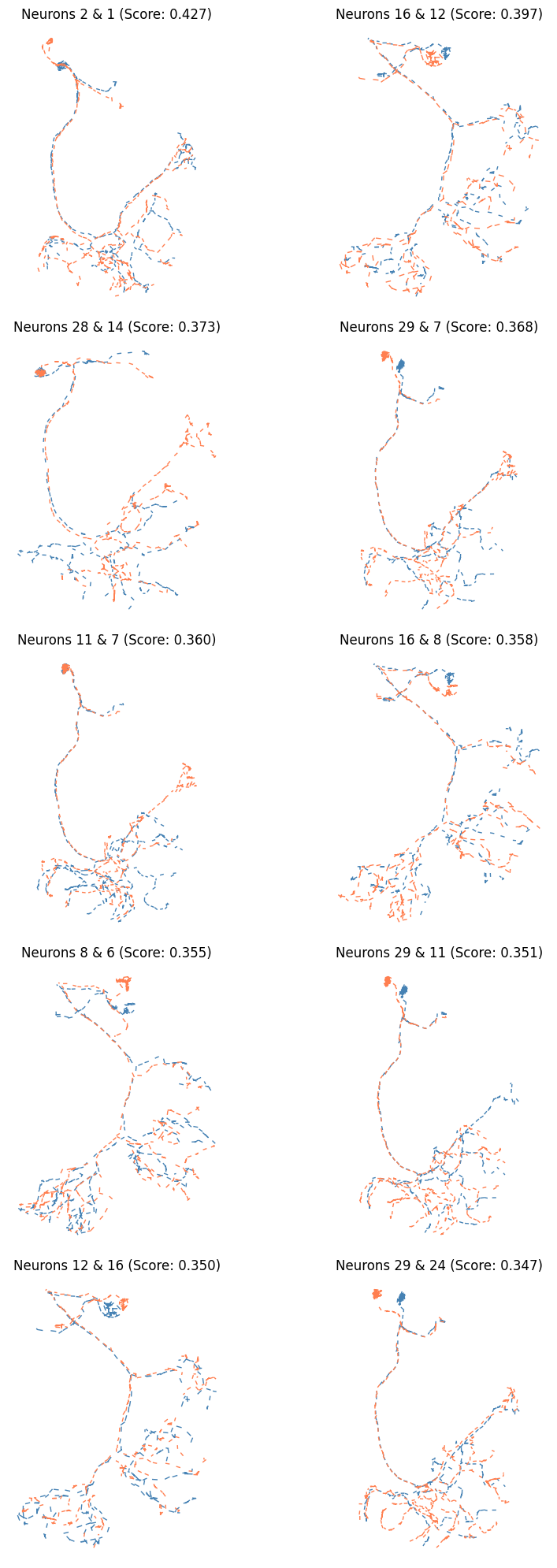
# plot the closest 10 pairs
closest_pairs = np.dstack(np.unravel_index(np.argsort(-scores.ravel()), scores.shape))[0][:10]
fig, axes = plt.subplots(5, 2, figsize=(10, 20))
for ax, (i, j) in zip(axes.ravel(), closest_pairs):
    navis.plot2d(dotprops[i], view=('x', 'y'), method='2d', ax=ax, color='steelblue')
    navis.plot2d(dotprops[j], view=('x', 'y'), method='2d', ax=ax, color='coral')
    ax.set_title(f'Neurons {i} & {j} (Score: {scores[i, j]:.3f})', fontsize=12)
    ax.grid(False)
    ax.set_axis_off()
plt.tight_layout()
plt.show()

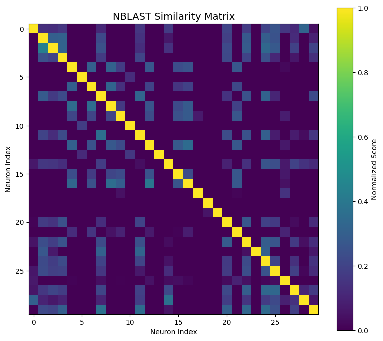
Most similar pair: neurons 2 and 1
Similarity score: 0.427

8. Distance Calculations

Understanding distances within neurons is crucial for many analyses. We’ll explore both Euclidean (straight-line) and geodesic (along-the-arbor) distances.

Sampling Rate (Node-to-Parent Distances)

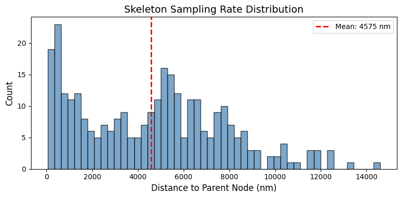
First, let’s calculate the average distance between nodes and their parents - this tells us about the skeleton’s sampling rate:

skel = l2_skels[0]

# Get nodes but remove the root (has no parent)
nodes = skel.nodes[skel.nodes.parent_id >= 0]

# Get the x/y/z coordinates of all nodes (except root)
node_locs = nodes[['x', 'y', 'z']].values

# For each node, get its parent's location
parent_locs = skel.nodes.set_index('node_id').loc[nodes.parent_id.values, ['x', 'y', 'z']].values

# Calculate Euclidean distances
distances = np.sqrt(np.sum((node_locs - parent_locs) ** 2, axis=1))

print(f"Sampling rate statistics:")
print(f"  Mean distance between nodes: {np.mean(distances):.2f} nm")
print(f"  Std: {np.std(distances):.2f} nm")
print(f"  Median: {np.median(distances):.2f} nm")

# Plot distribution
plt.figure(figsize=(8, 4))
plt.hist(distances, bins=50, color='steelblue', edgecolor='black', alpha=0.7)
plt.xlabel('Distance to Parent Node (nm)', fontsize=12)
plt.ylabel('Count', fontsize=12)
plt.title('Skeleton Sampling Rate Distribution', fontsize=14)
plt.axvline(np.mean(distances), color='red', linestyle='--', linewidth=2, label=f'Mean: {np.mean(distances):.0f} nm')
plt.legend()
plt.tight_layout()
plt.show()

Sampling rate statistics:
  Mean distance between nodes: 4575.27 nm
  Std: 3191.86 nm
  Median: 4793.04 nm

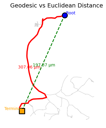
Geodesic Distance: Single Node-to-Node Query

For distances along the neuron’s branching structure, we need geodesic distances. Let’s calculate the distance from the soma (root) to a terminal node:

# Pick a terminal node
end_nodes = skel.nodes[skel.nodes.type == 'end'].node_id.values
terminal_node = end_nodes[0]

# Calculate geodesic distance from root to terminal node
d_geo = navis.dist_between(skel, skel.root[0], terminal_node)

# Also calculate Euclidean distance for comparison
end_loc = skel.nodes.set_index('node_id').loc[terminal_node, ['x', 'y', 'z']].values
root_loc = skel.nodes.set_index('node_id').loc[skel.root[0], ['x', 'y', 'z']].values
d_eucl = np.sqrt(np.sum((end_loc - root_loc) ** 2))

print(f"Distance from root to terminal node {terminal_node}:")
print(f"  Geodesic (along arbor): {d_geo:.2f} nm ({d_geo/1000:.2f} μm)")
print(f"  Euclidean (straight line): {d_eucl:.2f} nm ({d_eucl/1000:.2f} μm)")
print(f"  Ratio (tortuosity): {d_geo/d_eucl:.2f}x")

Distance from root to terminal node 5:
  Geodesic (along arbor): 307062.21 nm (307.06 μm)
  Euclidean (straight line): 197367.96 nm (197.37 μm)
  Ratio (tortuosity): 1.56x

# Visualize the difference between geodesic and Euclidean distances

# Find the shortest path along the skeleton
path = nx.shortest_path(skel.graph.to_undirected(), skel.root[0], terminal_node)

# Get coordinates for the path
path_co = skel.nodes.set_index('node_id').loc[path, ['x', 'y', 'z']].copy()

# Plot the neuron
fig, ax = navis.plot2d(skel, color='lightgray', method='2d', view=('x', 'y'), figsize=(5, 5))

# Add geodesic path (along the skeleton)
ax.plot(path_co.x, path_co.y, color='red', linewidth=3, label='Geodesic path', zorder=10)

# Add Euclidean path (straight line)
ax.plot([root_loc[0], end_loc[0]], [root_loc[1], end_loc[1]], 
        color='green', linewidth=2, linestyle='--', label='Euclidean path', zorder=10)

# Mark root and terminal node
ax.scatter(root_loc[0], root_loc[1], s=150, color='blue', marker='o', 
           label='Root (soma)', zorder=15, edgecolors='black', linewidths=2)
ax.scatter(end_loc[0], end_loc[1], s=150, color='orange', marker='s', 
           label='Terminal node', zorder=15, edgecolors='black', linewidths=2)

# Add text annotations
ax.text(root_loc[0], root_loc[1], ' Root', color='blue', fontsize=10, verticalalignment='bottom', horizontalalignment='left', zorder=20)
ax.text(end_loc[0], end_loc[1], ' Terminal', color='orange', fontsize=10, verticalalignment='bottom', horizontalalignment='right', zorder=20)   

# add distance annotations
mid_geo = path_co.iloc[len(path_co)//2]
mid_eucl = [(root_loc[0] + end_loc[0]) / 2, (root_loc[1] + end_loc[1]) / 2]
ax.text(mid_geo.x, mid_geo.y, f' {d_geo/1000:.2f} μm', color='red', fontsize=10, verticalalignment='bottom', horizontalalignment='center', zorder=20)
ax.text(mid_eucl[0], mid_eucl[1], f' {d_eucl/1000:.2f} μm', color='green', fontsize=10, verticalalignment='top', horizontalalignment='center', zorder=20)        

ax.set_title('Geodesic vs Euclidean Distance', fontsize=14)
ax.set_axis_off()
plt.show()

Geodesic Distance Matrix

For analyzing distances across many nodes, we can use navis.geodesic_matrix() to compute a distance matrix. Let’s calculate distances between all terminal nodes:

# Calculate distances from all end nodes to all other nodes
ends = skel.nodes[skel.nodes.type == 'end'].node_id.values
print(f"Calculating geodesic distances for {len(ends)} terminal nodes...")

# Get the distance matrix
dist_matrix = navis.geodesic_matrix(skel, from_=ends)

# Subset to only end-to-end distances
dist_matrix_ends = dist_matrix.loc[ends, ends]

print(f"\nDistance matrix shape: {dist_matrix_ends.shape}")
print(f"Distance statistics (μm):")
print(f"  Mean: {dist_matrix_ends.values.mean()/1000:.2f}")
print(f"  Median: {np.median(dist_matrix_ends.values)/1000:.2f}")
print(f"  Max: {dist_matrix_ends.values.max()/1000:.2f}")

display(dist_matrix_ends.head())

Calculating geodesic distances for 97 terminal nodes...

Distance matrix shape: (97, 97)
Distance statistics (μm):
  Mean: 194.81
  Median: 219.03
  Max: 379.44

	5	6	7	8	44	12	19	10	39	42	...	286	282	281	289	290	304	301	307	305	306
5	0.000000	1470.138794	21770.945312	21924.505859	43284.164062	82830.328125	68335.960938	162903.531250	155059.750000	97709.773438	...	196621.8750	194101.625000	194177.703125	213741.078125	215143.28125	214334.812500	206430.062500	228993.875000	230859.656250	229488.406250
6	1470.138794	0.000000	21653.496094	21807.058594	43166.718750	82712.882812	68218.515625	162786.093750	154942.312500	97592.328125	...	196504.4375	193984.187500	194060.265625	213623.640625	215025.84375	214217.375000	206312.625000	228876.437500	230742.218750	229370.968750
7	21770.945312	21653.496094	0.000000	963.262634	22322.921875	61869.085938	47374.718750	141942.296875	134098.500000	76748.531250	...	175660.6250	173140.375000	173216.468750	192779.843750	194182.03125	193373.578125	185468.812500	208032.625000	209898.406250	208527.156250
8	21924.505859	21807.058594	963.262634	0.000000	22476.482422	62022.648438	47528.281250	142095.859375	134252.062500	76902.093750	...	175814.1875	173293.937500	173370.031250	192933.406250	194335.59375	193527.140625	185622.375000	208186.187500	210051.968750	208680.718750
44	43284.164062	43166.718750	22322.921875	22476.482422	0.000000	58810.382812	44316.015625	138883.593750	131039.796875	73689.828125	...	172601.9375	170081.671875	170157.750000	189721.125000	191123.34375	190314.875000	182410.109375	204973.921875	206839.703125	205468.453125

5 rows × 97 columns

# Visualize the distance matrix with hierarchical clustering
from scipy.cluster.hierarchy import linkage
from scipy.spatial.distance import squareform

# Generate linkage from the distances
Z = linkage(squareform(dist_matrix_ends.values/1000, checks=False), method='ward')

# Create clustermap
fig = plt.figure(figsize=(10, 8))
cm = sns.clustermap(
    dist_matrix_ends.values/1000,  # Convert to microns
    cmap='viridis',
    col_linkage=Z,
    row_linkage=Z,
    cbar_kws={'label': 'Distance (μm)'},
    figsize=(10, 8)
)

cm.ax_heatmap.set_xlabel('Terminal Node', fontsize=12)
cm.ax_heatmap.set_ylabel('Terminal Node', fontsize=12)
cm.ax_heatmap.set_title('Geodesic Distances Between Terminal Nodes', fontsize=14, pad=150)

# Remove tick labels for cleaner look
cm.ax_heatmap.set_xticks([])
cm.ax_heatmap.set_yticks([])

plt.show()

print("\nNote: Clustering in the heatmap can reveal dendritic vs axonal compartments!")
print("Nodes that cluster together are likely in the same compartment.")

<Figure size 1000x800 with 0 Axes>

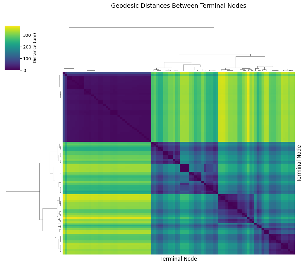
Note: Clustering in the heatmap can reveal dendritic vs axonal compartments!
Nodes that cluster together are likely in the same compartment.

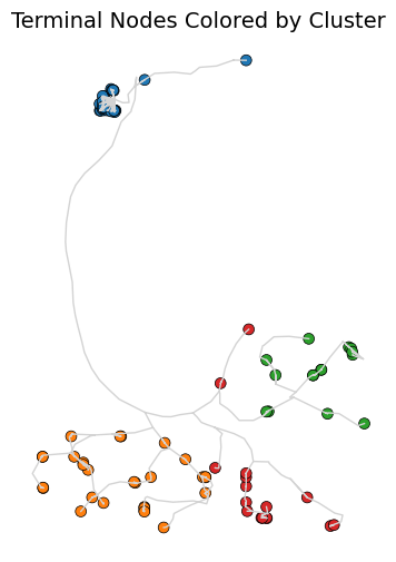
# get the clusters and plot them on the neuron
from scipy.cluster.hierarchy import fcluster
# Cut the dendrogram to form 2 clusters
clusters = fcluster(Z, t=4, criterion='maxclust')

# plot all the nodes colored by cluster
fig, ax = navis.plot2d(skel, method='2d', view=('x', 'y'), color='lightgray', figsize=(6, 6))
node_colors = sns.color_palette('tab10', n_colors=max(clusters)).as_hex()
node_colors = [node_colors[c-1] for c in clusters]
ax.scatter(
    skel.nodes.set_index('node_id').loc[ends, 'x'],
    skel.nodes.set_index('node_id').loc[ends, 'y'],
    c=node_colors, s=50, edgecolors='black', linewidths=0.5, label='Terminal Nodes'
)
ax.set_title('Terminal Nodes Colored by Cluster', fontsize=14)
ax.set_axis_off()
plt.show()

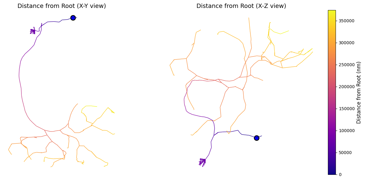
Distance-based Node Coloring

We can also use distances to color the neuron, highlighting how far each node is from the root:

# Calculate distance from root to all nodes
root_node = skel.root[0]
all_node_ids = skel.nodes.node_id.values
distances_all = navis.geodesic_matrix(skel, from_=all_node_ids)

# Add to nodes dataframe
skel.nodes['root_dist'] = distances_all.loc[root_node, :].values

# set nan to 0 
skel.nodes['root_dist'] = skel.nodes['root_dist'].fillna(0)

print(f"Distance from root statistics:")
print(f"  Mean: {skel.nodes['root_dist'].mean()/1000:.2f} μm")
print(f"  Max: {skel.nodes['root_dist'].max()/1000:.2f} μm")
print(f"  Std: {skel.nodes['root_dist'].std()/1000:.2f} μm")

# Plot neuron colored by distance from root
fig, axes = plt.subplots(1, 2, figsize=(14, 6))

# View 1: X-Y
navis.plot2d(
    skel,
    color_by='root_dist',
    palette='plasma',
    method='2d',
    view=('x', 'y'),
    ax=axes[0]
)
# plot the root
axes[0].scatter(
    root_loc[0], root_loc[1],
    color='blue', s=120, edgecolors='black', linewidths=2, label='Root'
)
axes[0].set_title('Distance from Root (X-Y view)', fontsize=14)
axes[0].set_axis_off()

# View 2: X-Z
navis.plot2d(
    skel,
    color_by='root_dist',
    palette='plasma',
    method='2d',
    view=('x', 'z'),
    ax=axes[1]
)
# plot the root
axes[1].scatter(
    root_loc[0], root_loc[2],
    color='blue', s=120, edgecolors='black', linewidths=2, label='Root'
)
axes[1].set_title('Distance from Root (X-Z view)', fontsize=14)
axes[1].set_axis_off()

# add colorbar
minimum = skel.nodes['root_dist'].min()
maximum = skel.nodes['root_dist'].max()
cbar = plt.colorbar(plt.cm.ScalarMappable(cmap='plasma', norm=plt.Normalize(vmin=minimum, vmax=maximum)), orientation='vertical', fraction=0.05, pad=0.1, cax=axes[1].inset_axes([1.05, 0, 0.05, 1]))
cbar.set_label('Distance from Root (nm)', fontsize=12)

plt.tight_layout()
plt.show()

Distance from root statistics:
  Mean: 236.91 μm
  Max: 374.03 μm
  Std: 101.03 μm

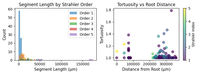
9. Advanced Morphometric Analysis

Segment Analysis

Navis provides segment_analysis() which collects comprehensive morphometrics for each linear segment (between branch points), including Strahler index, cable length, distance to root, and tortuosity.

# need to reroot the skeleton to the soma location
for i in range(3):
    skel = l2_skels[i]
    coords = soma_coords_batch[i] * scaling_factors  # scale to microns
    node_positions = skel.nodes[['x', 'y', 'z']].values
    dists = np.linalg.norm(node_positions - coords, axis=1)
    nearest_node_idx = np.argmin(dists)
    nearest_node_id = skel.nodes.iloc[nearest_node_idx]['node_id']
    print(f"Rerooting skeleton {skel.id} at nearest node {nearest_node_id} to soma location {coords} at distance {dists[nearest_node_idx]:.2f} microns")
    skel.reroot(nearest_node_id, inplace=True)

Rerooting skeleton 576460752700282748 at nearest node 223 to soma location [299120 250048  59514] at distance 1136.51 microns
Rerooting skeleton 576460752681552812 at nearest node 276 to soma location [294800 231440  83664] at distance 346.00 microns
Rerooting skeleton 576460752722405178 at nearest node 239 to soma location [289624 251488  85596] at distance 516.06 microns

# Perform comprehensive segment analysis
seg_analysis = navis.segment_analysis(l2_skels[0])

print(f"Segment analysis results:")
print(f"  Total segments: {len(seg_analysis)}")
print(f"\nFirst few segments:")
display(seg_analysis.head())

print(f"\nSummary statistics:")
display(seg_analysis[['length', 'tortuosity', 'root_dist', 'strahler_index']].describe())

Segment analysis results:
  Total segments: 152

First few segments:

	length	tortuosity	root_dist	strahler_index	radius_mean	radius_min	radius_max	volume
0	793.792721	1.009957	306268.419732	1	221.333333	193	244	1.326052e+08
1	20572.301259	1.093203	285696.118473	2	271.000000	193	314	5.024232e+09
2	676.346065	1.000000	306268.419732	1	191.000000	189	193	7.751780e+07
3	12285.961101	1.034210	273410.157373	2	212.750000	117	314	9.929913e+08
4	404.850590	1.000000	285696.118473	1	243.000000	172	314	7.724016e+07

Summary statistics:

	length	tortuosity	root_dist	strahler_index
count	152.000000	152.000000	152.000000	152.000000
mean	9270.934315	1.037665	225768.867012	1.513158
std	16940.222298	0.100488	106298.128510	0.813681
min	55.172457	1.000000	0.000000	1.000000
25%	1192.933156	1.000000	80607.110184	1.000000
50%	4983.385660	1.000000	265986.027429	1.000000
75%	10191.787491	1.024821	306346.790386	2.000000
max	173550.345434	1.788708	360682.099962	5.000000

# Visualize segment properties
seg_analysis = navis.segment_analysis(l2_skels[0])

fig, axes = plt.subplots(1, 2, figsize=(8, 3))

# Segment length distribution by Strahler order
for order in sorted(seg_analysis['strahler_index'].unique()):
    data = seg_analysis[seg_analysis['strahler_index'] == order]['length']
    axes[0].hist(data, bins=15, alpha=0.6, label=f'Order {int(order)}')
axes[0].set_xlabel('Segment Length (μm)', fontsize=11)
axes[0].set_ylabel('Count', fontsize=11)
axes[0].set_title('Segment Length by Strahler Order', fontsize=12)
axes[0].legend()

# Tortuosity vs distance from root
scatter = axes[1].scatter(
    seg_analysis['root_dist'], 
    seg_analysis['tortuosity'],
    c=seg_analysis['strahler_index'],
    cmap='viridis',
    s=50,
    alpha=0.6
)
axes[1].set_xlabel('Distance from Root (μm)', fontsize=11)
axes[1].set_ylabel('Tortuosity', fontsize=11)
axes[1].set_title('Tortuosity vs Root Distance', fontsize=12)
plt.colorbar(scatter, ax=axes[1], label='Strahler Index')

plt.tight_layout()
plt.show()

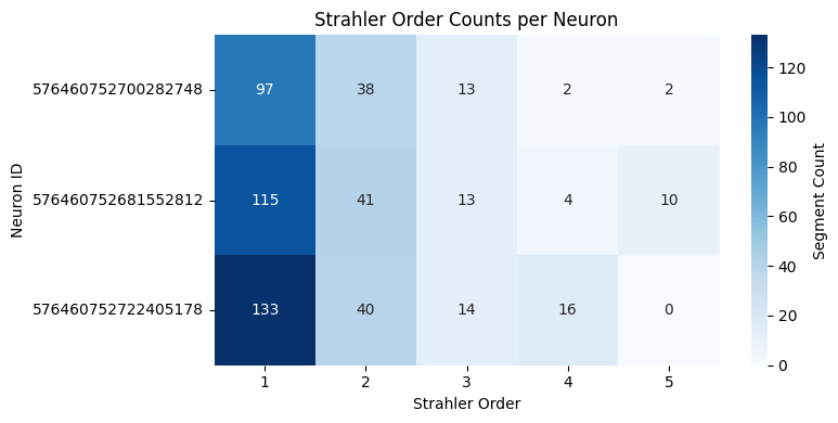
# compare strahler order counts between neurons

# calculate strahler order counts for each neuron
strahler_counts = []
for skel in l2_skels:
    seg_analysis = navis.segment_analysis(skel)
    counts = seg_analysis['strahler_index'].value_counts().to_dict()
    counts['root_id'] = skel.id
    strahler_counts.append(counts)
strahler_df = pd.DataFrame(strahler_counts).fillna(0).set_index('root_id').astype(int)

# show as a heatmap
plt.figure(figsize=(8, 4))
sns.heatmap(strahler_df, annot=True, fmt='d', cmap='Blues', cbar_kws={'label': 'Segment Count'})
plt.title('Strahler Order Counts per Neuron')
plt.xlabel('Strahler Order')
plt.ylabel('Neuron ID')
plt.tight_layout()
plt.show()

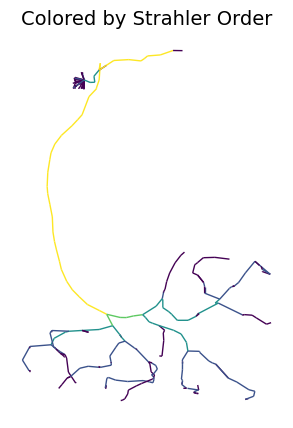
Visualizing Node Properties

# add strahler index to skeleton nodes
navis.strahler_index(l2_skels[0])

# Color by Strahler order
fig, ax = navis.plot2d(
    l2_skels[0],
    view=('x', 'y'),
    color_by='strahler_index',
    palette='viridis',
    method='2d',
    figsize=(5, 5)
)
ax.grid(False)
ax.set_title('Colored by Strahler Order', fontsize=14)
ax.set_axis_off()
plt.show()

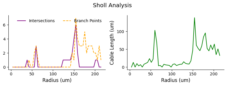
Sholl analysis

Sholl analysis quantifies branching complexity as a function of distance from the soma.

Euclidean distance from soma

Typically, Sholl analysis is performed using Euclidean distance from the soma.

# perform sholl analysis with euclidean radii of 50 nm increments from the root
sholl_results = navis.sholl_analysis(l2_skels[0], radii=50, center='root')
display(sholl_results.head())

# plot sholl results
fig, ax = plt.subplots(1,2, figsize=(8, 3))
ax[0].plot(sholl_results.index/1000, sholl_results['intersections'].values, ls ='-', color='purple', label='Intersections')
ax[0].plot(sholl_results.index/1000, sholl_results['branch_points'].values, ls='--', color='orange', label='Branch Points')
ax[0].set_xlabel('Radius (um)', fontsize=12)
ax[0].spines[['top', 'right']].set_visible(False)
ax[0].legend(frameon=False, ncols = 2)

ax[1].plot(sholl_results.index/1000, sholl_results['cable_length'].values/1000, ls='-', color='green')
ax[1].set_xlabel('Radius (um)', fontsize=12)
ax[1].set_ylabel('Cable Length (um)', fontsize=12)
ax[1].spines[['top', 'right']].set_visible(False)

plt.suptitle('Sholl Analysis', fontsize=14)
plt.tight_layout()

	intersections	cable_length	branch_points
radius
4283.629551	0	0.000000	0
8567.259101	0	13065.068359	0
12850.888652	0	0.000000	0
17134.518202	0	9701.698242	0
21418.147753	0	3230.100830	0

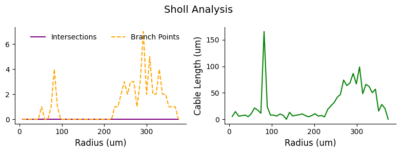
Geodesic distance from soma

Sholl analysis can also be performed using geodesic distance along the neuron structure.

# perform sholl analysis with euclidean radii of 50 nm increments from the root
sholl_results = navis.sholl_analysis(l2_skels[0], radii=50, center='root', geodesic=True)
display(sholl_results.head())

# plot sholl results
fig, ax = plt.subplots(1,2, figsize=(8, 3))
ax[0].plot(sholl_results.index/1000, sholl_results['intersections'].values, ls ='-', color='purple', label='Intersections')
ax[0].plot(sholl_results.index/1000, sholl_results['branch_points'].values, ls='--', color='orange', label='Branch Points')
ax[0].set_xlabel('Radius (um)', fontsize=12)
ax[0].spines[['top', 'right']].set_visible(False)
ax[0].legend(frameon=False, ncols = 2)

ax[1].plot(sholl_results.index/1000, sholl_results['cable_length'].values/1000, ls='-', color='green')
ax[1].set_xlabel('Radius (um)', fontsize=12)
ax[1].set_ylabel('Cable Length (um)', fontsize=12)
ax[1].spines[['top', 'right']].set_visible(False)

plt.suptitle('Sholl Analysis', fontsize=14)
plt.tight_layout()

	intersections	cable_length	branch_points
radius
7480.571289	0	5413.287598	0
14961.142578	0	14514.019531	0
22441.714844	0	6069.560547	0
29922.285156	0	6710.543457	0
37402.855469	0	8032.163574	0

Summary

In this comprehensive deep dive, you learned:

✅ Mesh representations - Fetching and analyzing neuron surface meshes
✅ Skeleton representations - Multiple methods (precomputed, L2-based)
✅ L2 graph analysis - High-quality morphology from L2 chunks
✅ Dotprops - Lightweight representations for fast comparisons
✅ Morphometric analysis - Cable length, branching, Strahler order, tortuosity
✅ Soma detection - Automated identification from mesh and skeleton data
✅ Visualization - 2D, 3D, and property-based coloring
✅ Population analysis - Comparing morphology across neuron groups
✅ Navis integration - Advanced analysis (NBLAST, resampling, smoothing)

Key Takeaways

1. Choose the right representation: Meshes for detail, skeletons for analysis, dotprops for comparison

2. L2-based morphology: Often more accurate than precomputed data

3. Fast estimates: Use get_l2_info() for quick morphology overview

4. Leverage navis: Full access to navis’s morphometric toolkit

5. Population studies: Compare morphology across cell types and conditions